Exploring Boston Open Crime Data with GGMap
Introduction
The Boston Crime Incidents Report is a dataset released by the city of Boston via the Boston open data portal which contains information about crimes reported to the BPD over the last few years (4/30/2011 - 6/03/2014).
The version of the dataset that I downloaded consists of 320,574 crimes reported during this period, and includes information about the nature of the incident (“Homicide”, “Larceny”, “Assault”, etc.), date & time of the report, as well as the location.
In this post, we’ll take a look at the geospatial aspect of the data, looking at how crime reports are geographically distributed in Boston.
Cleaning Up the Data
To start, let’s take a closer look at the data set. Here is a look at some of the columns in the data set and the first few records in the table:
> crime <- read.csv("Crime_Incident_Reports.csv")
> colnames(crime)
> [1] "COMPNOS" "NatureCode"
>  [3] "INCIDENT_TYPE_DESCRIPTION" "MAIN_CRIMECODE"
>  [5] "REPTDISTRICT" "REPORTINGAREA"
>  [7] "FROMDATE" "WEAPONTYPE"
>  [9] "Shooting" "DOMESTIC"
> [11] "SHIFT" "Year"
> [13] "Month" "DAY_WEEK"
> [15] "UCRPART" "X"
> [17] "Y" "STREETNAME"
> [19] "XSTREETNAME" "Location"
> head(crime)

    COMPNOS NatureCode INCIDENT_TYPE_DESCRIPTION MAIN_CRIMECODE

1 110220085 MVANO MVAcc MVAcc
2 110219791 CARST DEATH INVESTIGATION 01INV
3 110219155 UNCONS MedAssist MedAssist
4 110219159 BEIP BENoProp BENoProp
5 110219167 NIDV OTHER LARCENY 06xx
6 110219169 PERGUN Argue Argue
REPTDISTRICT REPORTINGAREA FROMDATE WEAPONTYPE Shooting
1 B2 320 04/30/2011 05:54:00 AM Unarmed No
2 A7 21 04/30/2011 06:00:00 AM Other No
3 E5 698 04/30/2011 06:21:00 AM Unarmed No
4 D4 620 04/30/2011 06:24:00 AM Unarmed No
5 B2 181 04/30/2011 06:50:00 AM Unarmed No
6 C11 351 04/30/2011 06:53:00 AM Firearm No
DOMESTIC SHIFT Year Month DAY_WEEK UCRPART X Y
1 No Last 2011 4 Saturday Part Three 768922.2 2938691
2 No Last 2011 4 Saturday Part Three 781735.0 2961811
3 No Last 2011 4 Saturday Part Three 751855.0 2928001
4 No Last 2011 4 Saturday Part Two 767168.1 2951333
5 Yes Last 2011 4 Saturday Part One 771778.9 2944026
6 No Last 2011 4 Saturday Part Three 775421.2 2934394
STREETNAME XSTREETNAME Location
1 HOWLAND ST WARREN ST (42.31116136, -71.08312956)
2 PARIS ST (42.37442134, -71.03529458)
3 W ROXBURY PY (42.28203873, -71.14639217)
4 HEMENWAY ST (42.34587634, -71.08938955)
5 GEORGE ST (42.32576135, -71.07246956)
6 SALISBURY PARK (42.29928135, -71.05918456)
We see that the data contains one record for each incident, as well as a number of other structured fields regarding the incident.
To plot the data on a map, we will make use of the “Location” field. However, we first need to convert this field into a more useful form–in particular, we need to split the latitude and longitude into two separate columns. To do this, we can use the stringr package with a bit of regex like so:
require(stringr)

> regex <-"\\((\\d+\\.\\d+), (-\\d+\\.\\d+)\\)"
> lat_long <- str_match(crime$Location, regex)[,2:3]
> lat_long <- apply(lat_long, 2, as.numeric)
> colnames(lat_long) <- c("y", "x")
> crime_latlong <- cbind(crime, lat_long)

> head(lat_long) #much better

            y         x

[1,] 42.31116 -71.08313
[2,] 42.37442 -71.03529
[3,] 42.28204 -71.14639
[4,] 42.34588 -71.08939
[5,] 42.32576 -71.07247
[6,] 42.29928 -71.05918
Exploring the Data with ggmap
With the location field cleaned up, we can now get to plotting. For this, we will use the ggmap package, which uses a ggplot-like grammar for easily plotting geospatial data. As a first exercise, here is the geographical distribution of drug charges in Boston:
# extract instances of drug charges

drug_crimes <- crime_latlong[crime_latlong$INCIDENT_TYPE_DESCRIPTION == "DRUG CHARGES",]

# plot on a map

require(ggmap)
map.center <- geocode("Boston, MA")
Bos_map <- qmap(c(lon=map.center$lon, lat=map.center$lat), zoom=12)
g <- Bos_map + geom_point(aes(x=x, y=y), data=drug_crimes, size=3, alpha=0.2, color="red") +
ggtitle("Drug Charges in Boston by Location (2011-2014)")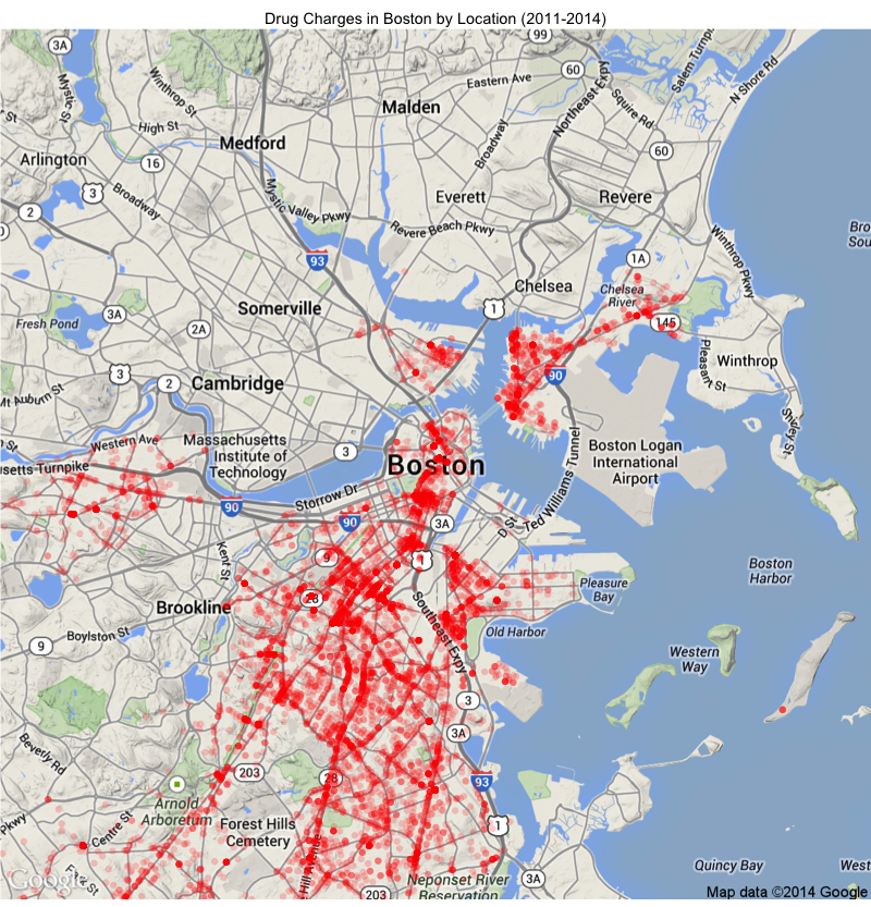
If you’re famililar with ggplot, you’ll note that ggmap is conceptually very similar. In this case Bos_map is my base layer map of Boston (centered on the lat-long determined by geocode). I then use geom_point to add the crime data layer to the map. If you want to learn more, a good introduction to ggmap can be found here.
As for the plot itself, a couple things are of note. For one thing, you may notice that a few regions of the city are conspicuously lacking in crime. In particular, there appear to have been exactly zero drug charges in Cambridge and Somerville over the last few years; likewise for Brookline. Of course this isn’t correct, but is rather a result of the fact that these areas are not part of the City of Boston proper, and hence were not included in the dataset (i.e. they have their own police departments).
To clarify this point, I thought it might make sense to visualize the exact geographic extent of the City of Boston. To do this, I pulled down the Boston Neighborhood Shapefiles from the open data portal. I have no previous experience working with shapefiles, but after a bit of googling (e.g.) and experimentation (and installing some new packages), I was able to plot them with ggmap:
#load R geo packages
require(rgdal)
require(sp)

#read the shape files
datadir <- "./Bos_neighborhoods_new/"
neighbs <- readOGR(dsn=datadir, layer="Bos_neighborhoods_new")

#prepare for plotting
neighbs <- spTransform(neighbs, CRS("+proj=longlat +datum=WGS84"))
neighbs_plt <- fortify(neighbs)

#plot the neighborhoods with ggmap
Bos_map2 <- qmap(c(lon=map.center$lon, lat=map.center$lat), zoom=11)
Bos_map2 + geom_polygon(data=neighbs_plt, aes(x=long, y=lat, group=group), alpha=0.3, color="black", fill='red') + ggtitle("Geographic Extent of Boston")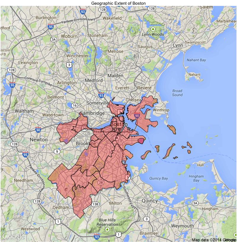
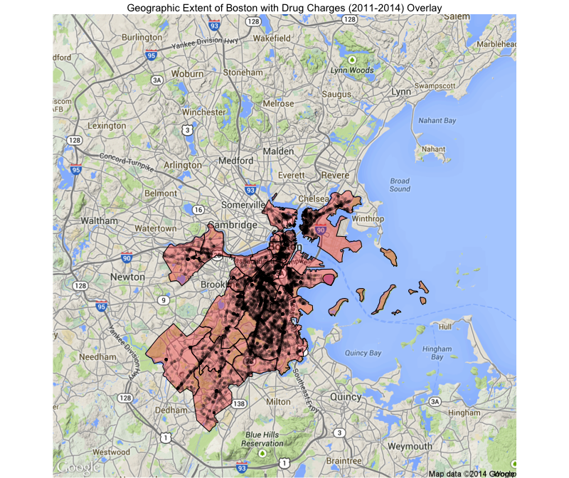
Each of the red-shaded polygons in this image represent a different neighborhood in the City of Boston. If we overlay this map with our previous drug charges plot, we see that, as expected, our dataset is entirely contained in this area (drug charges now represented in black):
# plot neighborhoods and crimes

Bos_map2 + geom_polygon(data=neighbs_plt, aes(x=long, y=lat, group=group), alpha=0.3, color="black", fill='red') +geom_point(aes(x=x, y=y), data=drug_crimes, size=2, alpha=0.2, color="black")+
ggtitle("Geographic Extent of Boston with Drug Charges (2011-2014) Overlay")