Notes on Stan and Price Comparison Modeling
Today, I am exploring the Stan “probabilistic programming language” for fitting Bayesian models. I have some formal background in Bayesian statistics (and implementing various related MCMC algorithms), but have not explored Stan much. I am interested in potentially using it for a research project, and so I will here explore it in that capacity by first outlining a theoretical economic model, and then testing approaches for estimating a parameter of interest (including using Stan).
Theory Setup
Here is the basic theoretical setup I want to explore.
Suppose that a consumer wants to purchase a good from one of two firms. Let $X_{1, i}$ and $X_{2,i}$ be the price of the good at firms 1 and 2 respectively for consumer $i$.
To start, let’s assume that $X_{1, i}$ and $X_{2, i}$ are both normally distributed and are independent (within and between different values of $i$):
\[X_{1, i} \sim N(\mu_1, \sigma^2_1)\] \[X_{2, i} \sim N(\mu_2, \sigma^2_2)\]Next, suppose that not all consumers compare prices. Let $\alpha$ be the probability that consumer $i$ compares prices on a given purchase decision. Let $R_i$ be a random indicator variable for whether consumer $i$ compares prices.
Next, let $Q_i$ be the final price paid by consumer $i$. Suppose that if the consumer does compare prices, the price they pay will be the minimum of the two available prices. In other words, if $R_i = 1$ then: $Q_i = \text{min}(X_{1, i}, X_{2, i})$. Otherwise, if $R_i = 0$, then the consumer will pay one of the prices at random: $Q_i = L_i (X_{1,i}) + (1-L_i)(X_{2,i})$, where $L_i$ is an indicator variable that is equal to 1 with probability $0.5$.
Supposing we observe some observations of $Q_i$ (but not the original prices), the question of interest for me is: what can we learn about $\alpha$, the rate of price comparison? To create the easiest starting point, let’s initially assume that $\mu_1, \sigma_1, \mu_2, \sigma_2$ are known. Specifically, suppose to start that: $\mu_1=20, \mu_2=15$, and $\sigma_1 = \sigma_2 = 3$.
Data Generating Process
Above, I’ve described the full data generating process, so in principle we should be able to write down the likelihood of the data we observe (i.e. observations of $Q_i$), given the other model parameters. The data generating process is:
- Draw $X_{1, i}\sim N(20, 9)$ and $X_{2, i}\sim N(15, 9)$
- Draw $R_i \sim Bern(\alpha)$
- Draw $L_i \sim Bern(0.5)$
- Compute $Q_i = R_i \text{min}(X_{1,i}, X_{2,i}) + (1-R_i)(L_iX_{1,i} + (1-L_i)X_{2,i})$.
To intuitively convince myself it is possible to learn about $\alpha$ given observations of $Q_i$, let’s run a simulation with a few different values of $\alpha$ and see how the distribution of $Q_i$ changes. First here is a function for one draw of $Q$ (for a choice of $\alpha$):
simulate_Q_once <- function(alpha, mu1, mu2, sd1, sd2) {
    # Step 1: Generate X1 and X2
    X1 <- rnorm(1, mean = mu1, sd = sd1)
    X2 <- rnorm(1, mean = mu2, sd = sd2)

    # Step 2: Generate R_i from a Bernoulli distribution with probability alpha
    R <- rbinom(1, size = 1, prob = alpha)

    # Step 3: Generate L_i from a Bernoulli distribution with probability 0.5
    L <- rbinom(1, size = 1, prob = 0.5)

    # Step 4: Compute F_i
    Q <- R*pmin(X1, X2)+(1-R)*(L*X1+(1 - L)*X2)

    return(Q)
}
Next, let’s run this function 5000 times for a range of different values of $\alpha$ and plot the results:
# Initialize a data frame to store the results

results <- data.frame(Q = numeric(), Alpha = factor())

# Define the alpha values and number of simulations

alpha_values <- c(0.25, 0.5, 0.75)
n_simulations <- 5000

# Perform simulations

for (alpha in alpha_values) {
    for (i in 1:n_simulations) {
        Q_draw <- simulate_Q_once(alpha, mu1=15, mu2=20, sd1=3, sd2=3)
        results <- rbind(results, data.frame(Q = Q_draw, Alpha = as.factor(alpha)))
    }
}
Here is a smoothed version of the resulting distributions:
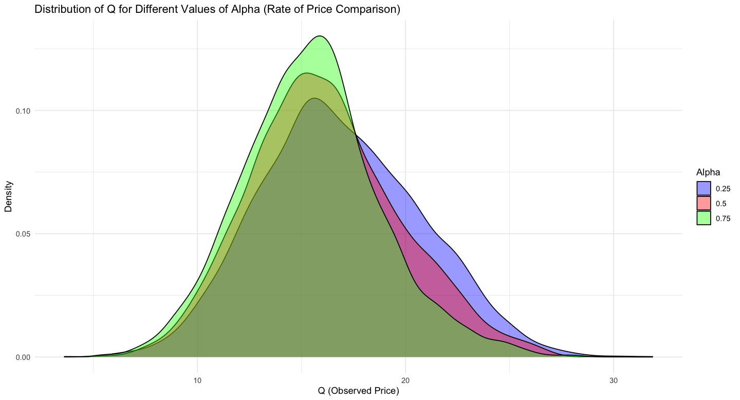
Likewise here are the estimated means and SDs of $Q$ under the different assumptions about $\alpha$:
| Alpha | Mean | SD |
|---|---|---|
| 0.25 | 16.777 | 3.866 |
| 0.5 | 16.031 | 3.687 |
| 0.75 | 15.438 | 3.330 |
What this all shows is that, as we anticipate, we generate different likelihoods for $Q$ under different values of $\alpha$. In particular, as $\alpha$ increases, $E[Q_i]$, the expected price paid, of course decreases. I also note that the shape of the distribution of $Q$ changes somewhat from something that is a mixture of two normals (no price comparison, random draw) to something that is the min of two normals. Of course all of this will depend on our assumptions about the initial price distributions. A good question is exactly what are the conditions under which $\alpha$ is identified, especially if we complicate the model.
Estimating Alpha from Moments
For now, let’s leave our assumptions as is and ask how we can recover $\alpha$ from our generated data. There are different approaches here. Recall that (suppressing the $i$ subscripts) we can write $Q$ as:
\[Q = R (\text{min}(X_1, X_2)) + (1-R)(L(X_{1}) + (1-L)(X_{2}))\]In this ultra simple version of the setup where the mean and SD of $X_1, X_2$ are fully known (and $E[L]=0.5$), we can recover $\alpha$ by taking expectations (relying on implicit independence assumptions and linearity):
\[E[Q] = E[R] E[(\text{min}(X_1, X_2))] + E[(1-R)](E[L]E[(X_{1}]) + E[(1-L)](E[X_{2}]))\] \[\rightarrow E[Q] = \alpha E[(\text{min}(X_1, X_2))] + (1-\alpha)(\frac{E[X_1]+E[X_2]}{2})\]Solving for $\alpha$ gives:
\[\alpha = \frac{E[Q]-\bar{\mu}}{E[\text{min}(X_1, X_2)] - \bar{\mu}}\]where $\bar{\mu} = (\mu_1 + \mu_2)/2.$ The only slightly complicated thing here is $E[\text{min}(X_1, X_2)]$; but this is just some integral that we can solve probably in closed form or with simulation if we are lazy. $E[Q]$ can then be estimated from the data and used to recover an estimate of $\alpha$; we could do this e.g. within a GMM framework (I think?) to get standard errors too.
For now, let’s test informally that it works using my simulated data with the true value of $\alpha = 0.25$, again under the assumption that $\mu_1=20, \mu_2=15$, and $\sigma_1 = \sigma_2 = 3$. From simulation, I find $E[\text{min}(X_1, X_2)] \approx 14.77$. From my simulated data, $E[Q] = 16.86$. Finally, $\bar{\mu} = (20+15)/2 = 17.5$. This implies estimate $\hat{\alpha}=0.231$ when $\alpha=0.25$. Checking my other cases, I find $\hat{\alpha}=0.502$ when $\alpha=0.5$, and $\hat{\alpha}=0.748$ when $\alpha=0.75$. So this all seems to work. It would be good practice to set this up in GMM and get standard errors, but I’ll leave that exercise for another time.
Estimating Alpha with Stan
With a view toward complicating our setup later on, I now want to try estimating $\alpha$ using a hierarchical modeling setup in Stan. In order to do this, the first thing we need to do is to write down the (log) likelihood of the data. Again, we start with:
\[Q = R (\text{min}(X_1, X_2)) + (1-R)(L(X_{1}) + (1-L)(X_{2}))\]What is an expression for $P(Q \leq q)$ – i.e. the CDF of $Q$? With a little algebra i find:
\[P(Q \leq q) = \alpha P(\text{min}(X_1, X_2) \leq q) + \frac{1-\alpha}{2} \left[P(X_1 \leq q) + P(X_2 \leq q)\right]\]What is $P(\text{min}(X_1, X_2) \leq q)$, the CDF of the min of two independent normals? From some basic manipulation we can show that:
\[P(\text{min}(X_1, X_2) \leq q) = P(X_1\leq q) + P(X_2\leq q) - P(X_1\leq q)P(X_2\leq q)\]These are all normal CDFs by assumption. Let $F_1$ and $F_2$ be the CDFs of $X_1$ and $X_2$; let $f_1$ and $f_2$ be the corresponding PDFs. Then the PDF of $\text{min}(X_1, X_2)$ (which I will call $f_m$) can be written as:
\[f_m(q) = f_1(q) + f_2(q) - [f_1(q)F_2(q) + F_1(q)f_2(q)].\]Likewise, we have that the PDF of $Q$ can be written as:
\[f_Q(q) = \alpha f_m(q) + \frac{1-\alpha}{2}(f_1(q) + f_2(q))\]So we have specified our likelihood. This is all tractable in principle because $X_1$ and $X_2$ are normals by assumption and so this is just some sums and products of normal PDFs and CDFs.
However, in Stan, we are encouraged to work on the log scale. So how can we express the log likelihood, $\log(f_Q(q))$? This gets a bit annoying because we have a number of sums in our likelihood expression. For working with logs of sums in Stan, it seems that using the “log-sum-exp” function is recommended. This trick involves writing:
\[\log(a+b) = \log(\exp(\log(a)) + \exp(\log(b)) := \text{log-sum-exp}(\log(a),\log(b))\]which I guess can be cleverly evaluated to avoid overflow/underflow issues. I will spare you the algebra; after a bunch of debugging, I come up with the following Stan script:
functions {
  // Log likelihood for the given complex density function
  real complex_log_likelihood(real q, real alpha, real mu1, real mu2, real sigma1, real sigma2) {

    real log_pdf_1 = normal_lpdf(q | mu1, sigma1);
    real log_pdf_2 = normal_lpdf(q | mu2, sigma2);
    real log_cdf_1 = normal_lcdf(q | mu1, sigma1);
    real log_cdf_2 = normal_lcdf(q | mu2, sigma2);

    // precompute some things
    real log_alpha = log(alpha);
    real log_one_minus_alpha = log(1-alpha);
    real log_f1q_plus_f2q = log_sum_exp(log_pdf_1, log_pdf_2);

    real log_fm_q = log(
        exp(log_pdf_1) + exp(log_pdf_2) - (exp(log_pdf_1)*exp(log_cdf_2) + exp(log_pdf_2)*exp(log_cdf_1))
    );

    real final = log_sum_exp(
        log_alpha + log_fm_q, log_one_minus_alpha - log(2) + log_f1q_plus_f2q
    );

    return(final);
  }
}
data {
    int<lower=0> N; // Number of observations
    vector[N] Q; // Observed prices
}
parameters {
    real<lower=0, upper=1> alpha; // P(price comparison)
}
model {
    real mu1=15;
    real mu2=20;
    real sigma1=3;
    real sigma2=3;

    for (i in 1:N) {
        target += complex_log_likelihood(Q[i],alpha, mu1, mu2, sigma1, sigma2);
    }
}
Note that stan implicitly is putting a $\text{Uniform}(0,1)$ prior on $\alpha$. I can of course test the sensitivity of results to this choice.
In any case, I run this via rstan for my various simulated data to see what I find in terms of posterior estimates for $\alpha$. I find that indeed, as desired, the posterior means are approximately equal to the true values of $\alpha$. Here is a plot of the posteriors:
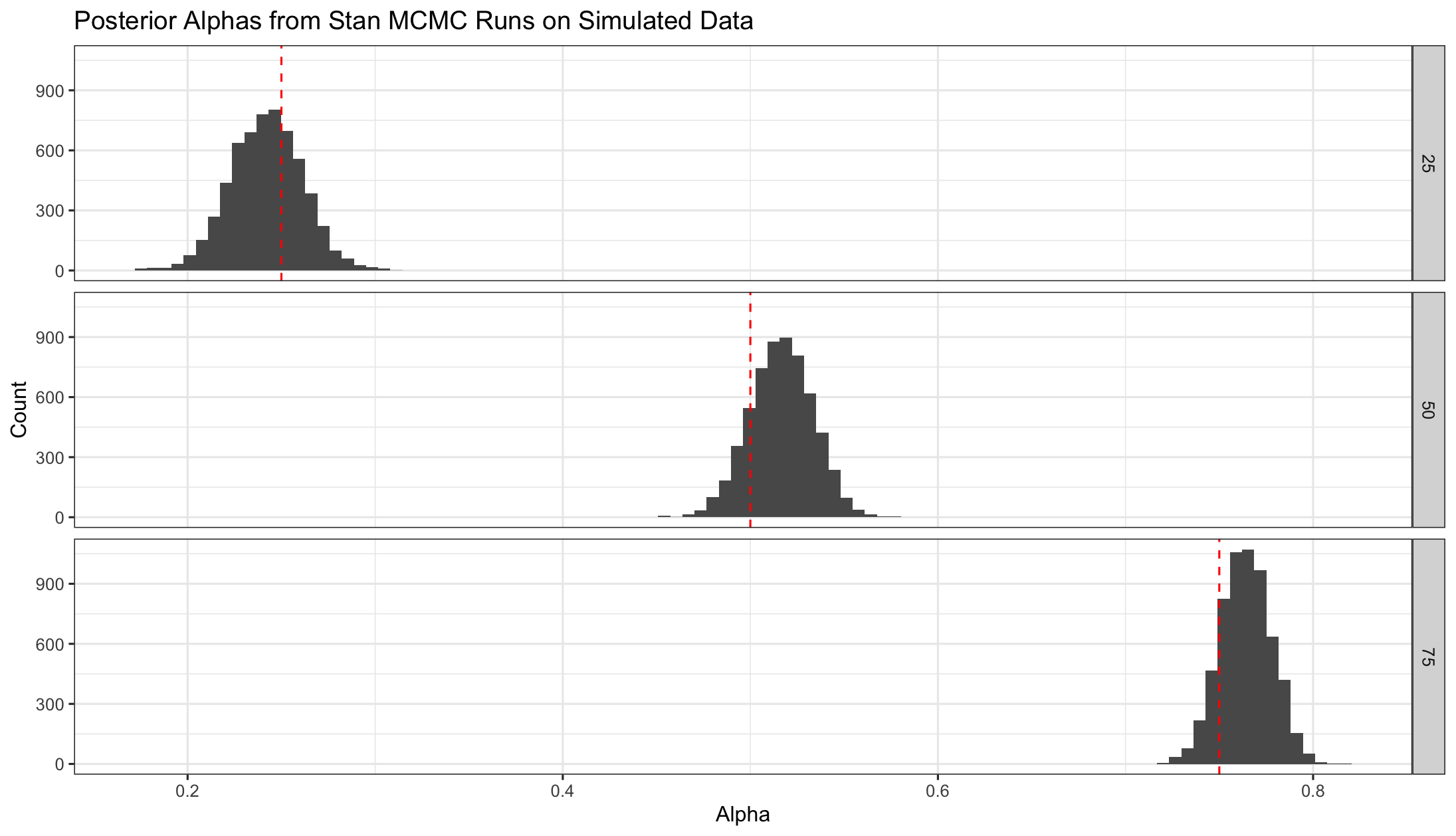
Here are the posterior means and bounds of 95% credible intervals (based on the quantiles of the simulated posteriors):
| True Alpha | Posterior Mean | 95% CI lower | 95% CI upper |
|---|---|---|---|
| 0.25 | 0.242 | 0.204 | 0.280 |
| 0.50 | 0.517 | 0.483 | 0.548 |
| 0.75 | 0.764 | 0.738 | 0.790 |
We see that in each case the credible interval covers the true $\alpha$ value from the simulation as we’d hope.
A Simple Generalization
Of course, given the likelihood, we could have estimated $\alpha$ in other ways too (e.g. MLE). However, the setup in Stan points allows for generalization that I am interested in developing. There’s a few steps I would like to take here.
However, for a simple generalization of the current setup, I will now consider the following: rather than assuming I exogenously know the parameters of the price distribution, I will put some priors on $\sigma_1, \sigma_2, \mu_1, \mu_2$, and assume that I observe some draws from the joint distribution of $(X_1, X_2)$ (still assuming independence for now). The stan code now looks like this (not reprinting the function block):
data {
    int<lower=0> N; // Number of observations
    vector[N] Q; // Observed prices
    int<lower=0> K; // Num of previous price obs
    vector[K] X1; // previous price obs
    vector[K] X2; // previous price obs
}
parameters {
    real<lower=0, upper=1> alpha; // P(price comparison)
    real<lower=0> mu1;
    real<lower=0> mu2;
    real<lower=0> sigma1;
    real<lower=0> sigma2;
}
model {

    X1 ~ normal(mu1, sigma1);
    X2 ~ normal(mu2, sigma2);

    for (i in 1:N) {
        target += complex_log_likelihood(Q[i],alpha, mu1, mu2, sigma1, sigma2);
    }
}
The data I feed as $X1$ and $X2$ are simply 1000 simulated draws from the true price distributions. Here are the results for the $\alpha=0.25$ case:
| mean | se_mean | sd | 2.5% | 50% | 97.5% | n_eff | |
|---|---|---|---|---|---|---|---|
| alpha | 0.24 | 0.00 | 0.03 | 0.19 | 0.24 | 0.30 | 2510 |
| mu1 | 15.02 | 0.00 | 0.07 | 14.88 | 15.02 | 15.16 | 3267 |
| mu2 | 19.99 | 0.00 | 0.08 | 19.82 | 20.00 | 20.15 | 3528 |
| sigma1 | 2.94 | 0.00 | 0.05 | 2.86 | 2.94 | 3.03 | 2646 |
| sigma2 | 2.93 | 0.00 | 0.05 | 2.84 | 2.93 | 3.03 | 2925 |
| lp__ | -16885.18 | 0.03 | 1.63 | -16889.29 | -16884.85 | -16883.06 | 2186 |
So we see that we still recover a reasonable estimate for $\alpha$, as well as for the other price parameters. Notably, the credible intervals for $\alpha$ are now somewhat wider. This makes sense given the added uncertainty we’ve introduced in the model.
What’s next?
So far, this is still pretty straightforward. However, it shows that we can estimate a price comparison rate given the following:
- Observations of paid prices.
- Some iid draws from the true price distributions (and parametric assumptions on these distributions)
- Assuming that consumers who price compare will always pay the lower price (while non-comparers will not).
What I am eventually interested in understanding is how price comparison rates vary across related markets which might have different characteristics, and under the setup that I may not observe true price draws from all markets (and so will need to do some partial pooling). The hope is to be able relate market characteristics to rates of price comparison, so that I can descriptively understand when consumers do or do not seem to be comparing prices. In the next section I will sketch this idea.
Many markets generalization (sketch)
Suppose that we now observe paid price data (i.e. $Q$) across $J$ markets over $T$ periods. So now, let $Q_{ijt}$ be an observed paid price for consumer $i$ in market $j$ in period $t$. We are now interested in estimates of $\alpha_{jt}$, the rate of price comparison in market $j$ during period $t$. The issue is that we will not necessarily observe true price data from all market-period cells (since data collection is costly). To address this, I will assume that the market-cell-level price distribution parameters are related in a hierarchical modeling setup, which allows me to infer something about the price distribution parameters of even unobserved market-period cells, and estimate $\alpha$ for these cases while accounting for this added uncertainty. If I then collect other information about the markets, I can examine how the $\alpha_{jt}$ estimates vary across market characteristics.